From Sequential Tests to Change Detections

Online change detection problem

The previous example illustrates a sub field of the statistical analysis called “online change detection problem”. Formally, suppose we have a stream of independent random observations \(X_1, X_2, \dots\). We know that under the normal condition, each observation follows a “pre-change” distribution \(P\). But if a change happens at an unknown time \(\nu \geq 0\) then after the time \(\nu\), each observation in the following sub-sequence \(X_{\nu+1}, X_{\nu+2}, \dots\) follows another “post-change” distribution \(Q\). Here \(\nu = 0\) implies the change happened at the very beginning so all observations follow the post-change distribution \(Q\). On the other hand, we set \(\nu = \infty\) to indicate a change never happens and all observations follow the pre-change distribution \(P\). The coin toss example above can be modeled by \(P = B(0.5)\) and \(Q = B(p)\) for some \(p \neq 0.5\). For a simple presentation, in this post we assume both pre- and post-change distributions \(P\) and \(Q\) are known to us in advance. ¹ Throughout this post, we refer \(\mathbb{E}_{\nu}\) to the expectation operator corresponding to the case where the change happened at time \(\nu \in \{0,1,\dots,\infty\}\).

The standard approach of the online change detection problem is to design a stopping time \(N\). If \(N < \infty\) then at the time \(N\), we declare a change happened before \(N\). One commonly used metric of the efficiency of the stopping time \(N\) is the worst average detection delay (WAD) conditioned on the detection time being later than the true change point that is defined by \[ \mathcal{J}(N) := \sup_{v\geq 0}\mathbb{E}_\nu \left[N - \nu | N > \nu\right]. \]

Note that the WAD is lower bounded by \(1\) and this lower bound can be easily achieved by setting \(N = 1\). That is, we just declare there was a change as soon as observing a single data point. If there was no change point then we can declare the change after observing another data point and so on.

Of course, this type of trivial change detector is far from ideal as it will trigger lots of false alerts at the highest possible frequency. In other words, this trivial change detector has the shortest run length, 1, until triggering a false alert. Therefore, when we design a change detector \(N\), we want the stopping time \(N\) to be able to detect the change as quickly as possible while controlling the false alert rate at a pre-defined rate. A commonly used metric for false alert rate is called the average run length (ARL) defined by the expectation of the stopping time of the change detector under the pre-change distribution. Formally, for a fixed constant \(\alpha \in (0,1)\), we call a stopping time \(N\) contols the ARL by \(1/\alpha\) if \[ \mathbb{E}_{\infty}[N] \geq 1/\alpha. \]

Building a change detector based on repeated sequential tests

So far, we have discussed how one can formulate the online change detection problem: Find a stopping time \(N\) minimizing the worst average detection delay (WAD), \(\mathcal{J}(N)\) while controlling average run length (ARL) by \(1/\alpha\), that is, \(\mathbb{E}_{0}[N] \geq 1/\alpha.\) But, how we can construct a such stopping time \(N\)? The Lorden’s lemma provides a simple way to convert any sequential testing method into an online change detector by proving a fact that repeated sequential tests can be viewed as an online change detection procedure.²

As a concrete example, let’s go back to the coin toss example. If we want to test whether a coin is fair (\(P = B(p),~~p =0.5\)) or biased toward the head (\(Q = B(q),~~q >0.5\)) with a level \(\alpha \in (0,1)\) then we can use the Wald’s SPRT, which is given by the following stopping time, \[ N := \inf\left\{n \geq 1: \sum_{i=1}^n \log\Lambda_i \geq \log(1/\alpha)\right\}, \] where each \(\Lambda_n\) is the likelihood ratio of \(P\) over \(Q\), which is given by \[ \Lambda_n := \left(\frac{q}{p}\right)^{X_n}\left(\frac{1-q}{1-p}\right)^{1-X_n}, \] for a sequence of Bernoulli observations \(X_1, X_2, \dots \in \{0,1\}\).

If the stopping time happen (\(N < \infty\)) then we stop and reject the null hypothesis, so we conclude the coin is biased toward the head. This sequential test controls the type-1 error by \(\alpha\) as we have \(P(N < \infty) \leq \alpha\).

Now, by using the Lorden’s lemma, we can convert this sequential test into a change detection procedure \(N^*\), which is given by \[\begin{align*} N^* &:= \min_{k \geq 1} \left\{N_k + k - 1\right\} \\ & = \inf\left\{n \geq 1: \max_{k \geq 1}\sum_{i=k}^n \log\Lambda_i \geq \log(1/\alpha)\right\}. \end{align*}\] If the stopping time \(N^*\) happen (\(N^* < \infty\)) then we stop and declare that we detect a change. Note that this change detection procedure is nothing but repeated Wald’s SPRT at each time \(k\). From the Lorden’s lemma, this online change detection procedure controls the ARL by \(1/\alpha\), that is, we have \(\mathbb{E}_{\infty}[N^*] \geq 1/\alpha\). In general, we cannot get the exact ARL control \(\mathbb{E}_{\infty}[N^*] = 1/\alpha\) by using the Lorden’s lemma. However, this method often performs almost as good as the optimal one. Especially for this Bernoulli case, if we replace the threshold \(\log(1/\alpha)\) with another constant \(a\) achieveing the exact ARL control then this procedure recovers the CUSUM procedrue which is known to be optimal procedure in this example.

Implementation

The change detection procedure \(N^*\) can be implemented in an online fashion as follows:

• Set \(M_0 := 0\)

• Update \(M_n := \max\{M_{n-1}, 0\} + \log \Lambda_n\)

• Make one of two following decisions:

  • If \(M_n \geq \log(1/\alpha)\) then stop and declare a change happened.
  • Otherwise, continue to the next iteration.

set.seed(1)
n_max <- 500L
# This memory is not required but only for the simple visualization.
m_vec <- numeric(n_max)
m <- 0
# Unbiased coin toss example
p_true <- 0.5
# Set up the baseline likelihood ratio
# Pre-change: p = 0.5
# Post-change: q = 0.6 
p <- 0.5
q <- 0.6
# ARL control at 1000
alpha <- 1e-3 
n_star <- Inf
not_yet_detected <- TRUE
for (i in 1:n_max) {
  # Observe a new coin toss
  x <- rbinom(1, 1, prob = p_true)
  # Update the change statistic
  m <- max(m, 0) + ifelse(x == 1, log(q/p), log((1-q)/(1-p)))
  # Check whether the stopping time happens
  if (m > log(1/alpha) & not_yet_detected) {
    n_star <- i
    not_yet_detected <- FALSE
    # For the normal implementation, we can stop at the stopping time
    # break
  }
  # Save the statistic for visualization
  m_vec[i] <- m
}
plot(1:n_max, m_vec, type = "l", xlab = "n", ylab = expression('M'['n']),
     ylim = c(0, 20))
abline(h = log(1/alpha), col = 2)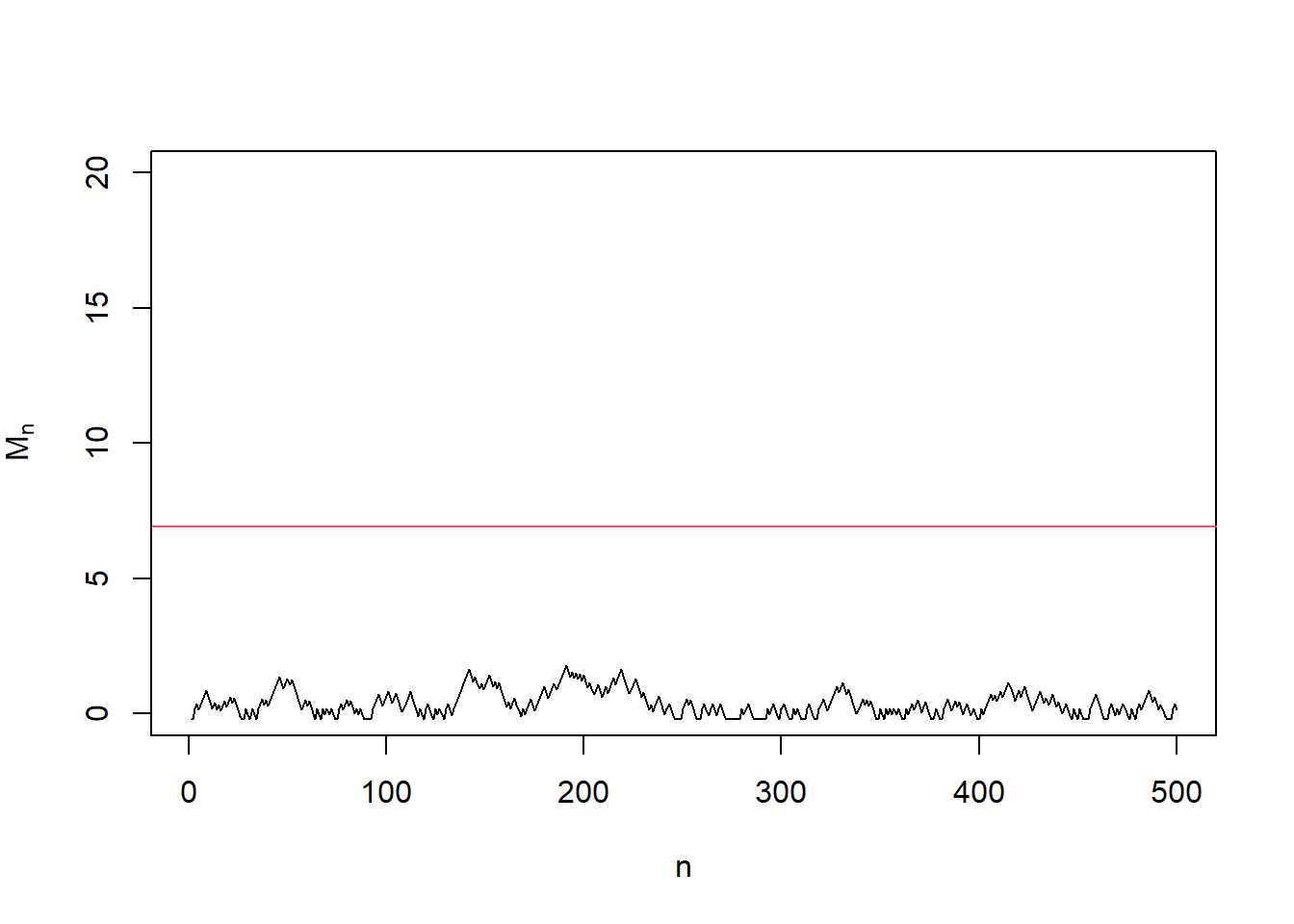

if (!is.infinite(n_star)) {
  abline(v = n_star, col = 2)
  print(paste0("Change detected at ", n_star))
} else {
  print("No change detected")
}

## [1] "No change detected"

set.seed(1)
n_max <- 500L
# This memory is not required but only for the simple visualization.
m_vec <- numeric(n_max)
m <- 0
# Biased coin toss example
p_pre <- 0.5
p_post <- 0.6
nu <- 200
# Set up the baseline likelihood ratio
# Pre-change: p = 0.5
# Post-change: q = 0.6 
p <- 0.5
q <- 0.6
# ARL control at 1000
alpha <- 1e-3 
n_star <- Inf
not_yet_detected <- TRUE
for (i in 1:n_max) {
  # Observe a new coin toss
  if (i < nu) {
    x <- rbinom(1, 1, prob = p_pre)
  } else {
    x <- rbinom(1, 1, prob = p_post)
  }
  # Update the change statistic
  m <- max(m, 0) + ifelse(x == 1, log(q/p), log((1-q)/(1-p)))
  # Check whether the stopping time happens
  if (m > log(1/alpha) & not_yet_detected) {
    n_star <- i
    not_yet_detected <- FALSE
    # For the normal implemenation, we can stop at the stopping time
    # break
  }
  # Save the statistic for visualization
  m_vec[i] <- m
}
plot(1:n_max, m_vec, type = "l", xlab = "n", ylab = expression('M'['n']),
     ylim = c(0, 20))
abline(h = log(1/alpha), col = 2)
abline(v = nu, col = 1)
if (!is.infinite(n_star)) {
  abline(v = n_star, col = 2)
  print(paste0("Change detected at ", n_star))
} else {
  print("No change detected")
}

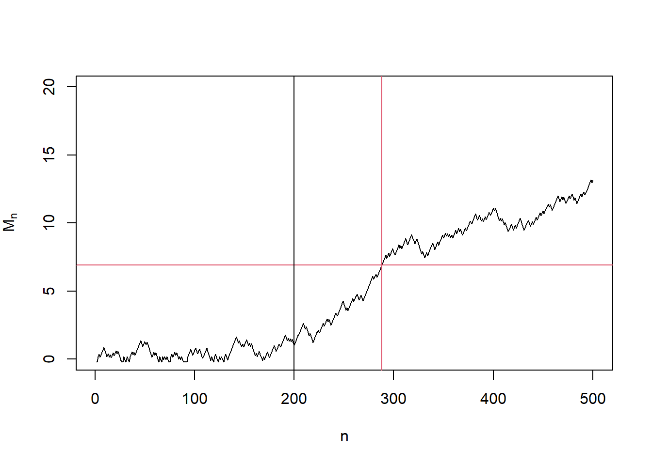
## [1] "Change detected at 288"

Conclusion

The Lorden’s lemma tells us that repeated sequential tests can be used as a change detection procedure. Therefore, whenever we can do a sequential test, we can do also a change detection procedure, which is useful to monitor a silent change in the underlying distribution.