Advantages of Sequential Hypothesis Testing: 2. Flexibility and Safety
In this follow-up post, we explain another advantage of sequential hypothesis testing: Flexibility and safety. Please visit the previous post for an introduction to Wald’s sequential probability ratio test (SPRT) and a discussion of its sample efficiency.
Can we early stop the testing if the p-value already reached below \(\alpha\)?
Again, let’s start with a simple coin toss example where we observe a sequence of independent observations \(X_1, X_2, \dots \in \{0,1\}\) from a Bernoulli distribution \(B(p)\) with \(p \in (0,1)\). We are interested in testing whether the underlying coin is pair (\(H_0: p = 0.5\)) or biased toward to head (\(H_1: p > 0.5\)).
From the previous post, we know that the binomial test is the best fixed sample size test. Formally, let’s set up the binomial test of level \(\alpha = 0.05\) with the minimum power of \(\beta = 0.95\) at \(p = 0.6\). In this case, the minimum sample size is given by the following R script.
set.seed(1)
printf <- function(...) invisible(print(sprintf(...)))
n_to_power <- function(n, p0, p1, alpha) {
  n <- ceiling(n)
  thres <- qbinom(alpha, n, p0, lower.tail = FALSE) # Reject null if s > thres
  pwr <- pbinom(thres, n, p1, lower.tail = FALSE)
  return(pwr)
}

power_to_n <- function(beta, p0, p1, alpha) {
  f <- function(n) {
    beta - n_to_power(n, p0, p1, alpha)
  }
  root <- stats::uniroot(f, c(1, 1e+4), tol = 1e-6)
  return(ceiling(root$root))
}

alpha <- 0.05
beta <- 0.95
p0 <- 0.5
p1 <- 0.6
n <- power_to_n(beta, p0 , p1 , alpha)
printf("%i is the minimum sample size to achieve test level %.2f and power %.2f at p= %.1f against the null p=%.2f.",
       n, alpha, beta, p1, p0)
## [1] "280 is the minimum sample size to achieve test level 0.05 and power 0.95 at p= 0.6 against the null p=0.50."In the standard fixed sample size setting, we compute the p-value once collecting all 280 samples. Then, if the p-value is less than the test level \(\alpha\), we reject the null hypothesis. In this case, we can control the type-1 error below \(\alpha\) and achieve the minimum power \(\beta\) under the alternative (\(p = 0.6\)), as the following simulation demonstrates.
binom_p_value <- function(s, n, p0) {
   return(pbinom(s-1, n, p0, lower.tail = FALSE))
}
run_binom_simul <- function(p_true, n, p0, alpha, max_iter) {
  # We shorten the simulation by using the fact X_1 + ...+X_n ~ Binom(n, p)
  s_vec <- rbinom(max_iter, size = n, prob = p_true)
  p_vec <- sapply(s_vec, binom_p_value, n = n, p0 = p0)
  return(mean(p_vec <= alpha))
}
# Under the null
max_iter <- 1e+4L
type_1_err <- run_binom_simul(p_true = p0, n, p0, alpha, max_iter)
printf("Type-1 error of the binomial test is %.2f.", type_1_err)
## [1] "Type-1 error of the binomial test is 0.04."# Under the alternative
pwr <- run_binom_simul(p_true = p1, n, p0, alpha, max_iter)
printf("Power of the binomial test at p=%.1f is %.2f.", p1, pwr)## [1] "Power of the binomial test at p=0.6 is 0.95."What if we observe the coin toss one by one and we compute the p-value at each time whenever a new coin toss happens? In the previous post, we noticed that Wald’s sequential probability ratio test (SPRT) can achieve a high sample efficiency by adaptively stopping the test procedure. Why not do the same trick to the binomial test? Can we early stop the testing if the p-value already reached below \(\alpha\)? Let’s run a simulation to check whether this early stopping still results in a type-1 error below the test level \(\alpha\).
run_binom_early_stop <- function(p_true, n, p0, alpha) {
  s <- 0
  for (i in 1:n) {
    s <- s + rbinom(1, size = 1, prob = p_true)
    p <-  binom_p_value(s, i, p0)
    if (p <= alpha) {
      return(TRUE)
    }
  }
  return(FALSE)
}
# Under the null
early_stopp_type_1_err <- mean(replicate(max_iter,{
  run_binom_early_stop(p_true = 0.5, n, p0, alpha)
  }))
printf("Type-1 error of the early stopped binomial test is %.2f.", early_stopp_type_1_err)
## [1] "Type-1 error of the early stopped binomial test is 0.26."It turns out that the early stopping strategy increased the type 1 error significantly above the target level. This inflation of type-1 error is an example of p-hacking. This issue is getting worse if we run a longer test.
set.seed(4)
s_vec <- cumsum(rbinom(n, size = 1, prob = 0.5))
f <- function(i) binom_p_value(s_vec[i], i, p0)
p_vec <- sapply(seq_along(s_vec), f)
plot(seq_along(p_vec), p_vec, type = "l", xlab= "n", ylab ="p-value")
abline(h = alpha, col = 2)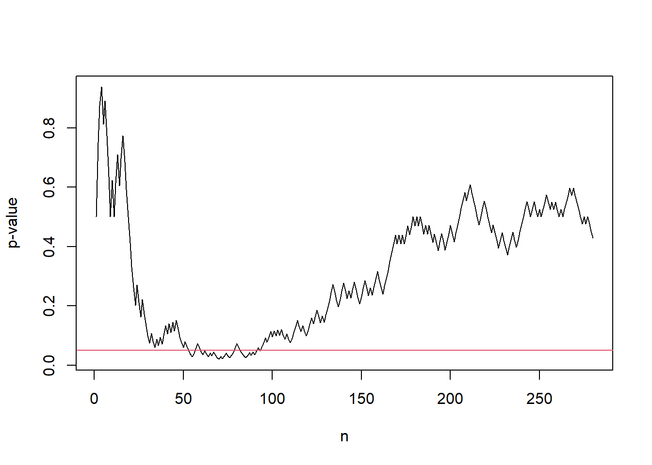 Fig. 1 An example sample path of p-values hitting the threshold \(\alpha\) although the underlying samples generated under the null. The red horizontal line corresponds to the test level \(\alpha\).
Can we continue to collect more samples if the p-value at the end is slightly above \(\alpha\)?
Okay, we learned that we should not early stop and wait to collect all samples of the pre-calculated size. But what if the p-value is slightly above \(\alpha = 0.05\) - let’s say \(p = 0.15\). Maybe, if we would have collected a bit more samples then the p-value might possibly be less than \(\alpha\) and we could reject the null. Can we continue to collect more samples to see whether the p-value becomes less than \(\alpha\) or goes away from it?
Let’s run a simple simulation to answer the question. For each run, we first collect the minimum sample size \(n\) computed to achieve the minimum power \(\beta = 0.95\). Then, compute the p-value based on the collected \(n\) samples. If the p-value is less than \(0.2\) then we collect another \(n\) samples and re-compute the p-value based on \(2n\) samples. Finally, we reject the null if the final p-value is less than or equal to the test level \(\alpha\).
run_binom_a_bit_more_simul <- function(p_true, n, p0, alpha, max_iter) {
  # We shorten the simulation by using the fact X_1 + ...+X_n ~ Binom(n, p)
  s_vec <- rbinom(max_iter, size = n, prob = p_true)
  p_vec <- sapply(s_vec, binom_p_value, n = n, p0 = p0)

  # If p-value > alpha and < 0.2, collect n more samples
  above_alpha_ind <- which(p_vec > alpha & p_vec < 0.2)
  s_vec[above_alpha_ind] <-
    s_vec[above_alpha_ind] + rbinom(length(above_alpha_ind), size = n, prob = p_true)
  p_vec[above_alpha_ind] <- sapply(s_vec[above_alpha_ind], binom_p_value, n = 2*n, p0 = p0)
  return(mean(p_vec <= alpha))
}
a_bit_more_type_1_err <- run_binom_a_bit_more_simul(p_true = p0, n, p0, alpha, max_iter)
printf("Type-1 error of the binomial test with the contional continuation is %.3f.", a_bit_more_type_1_err)
## [1] "Type-1 error of the binomial test with the contional continuation is 0.063."In this case, the type-1 error increased above the test level \(\alpha\) though it is not as dramatic as the early stopping case. If we continuously collect and compute p-values rather than collect a single batch then the inflation of the type-1 error becomes more significant. This type of continuation of the testing procedure is also an example of p-hacking.
run_binom_a_bit_more2_run <- function(p_true, n, p0, alpha) {
  s <- rbinom(1, size = n, prob = p_true)
  p <-  binom_p_value(s, n, p0)
  if (p <= alpha) {
    # If first n samples give p-value less than alpha
    # Reject the null
    return(TRUE)
  } else if (p >= 0.2) {
    # If first n samples give p-value above 0.2
    # Fail to reject the null and stop the test
    return(FALSE)
  }
  # Otherwise, continue the test until we collect another n samples.
  for (i in 1:n) {
    s <- s + rbinom(1, size = 1, prob = p_true)
    p <-  binom_p_value(s, i, p0)
    if (p <= alpha) {
      return(TRUE)
    }
  }
  return(FALSE)
}
# Under the null
a_bit_more2_type_1_err <- mean(replicate(max_iter,{
  run_binom_a_bit_more2_run(p_true = 0.5, n, p0, alpha)
  }))
printf("Type-1 error of the binomial test with the additional continous monitoring is %.2f.", a_bit_more2_type_1_err)
## [1] "Type-1 error of the binomial test with the additional continous monitoring is 0.18."Always-valid p-values - flexibly and safely early stop or continue the test.
So far, we have observed how the early stop or continual test results in the type-1 error inflation for fixed sample size tests. The root cause of this inflation is that the p-value from a fixed sample size test is valid only at the pre-specified fixed sample size. In other words, let \(p_n\) be the p-value of \(n\) samples. Then we have \[ P_{H_0}\left(p_n \leq \alpha\right) \leq \alpha, ~~\forall n. \] However, to early stop or continue the test without the type-1 error inflation, we need the following stronger inequality. \[ P_{H_0}\left(\exists n: p_n \leq \alpha\right) \leq \alpha. \] Note that fixed sample based p-values do not necessarily satisfy the above strong inequality.1
If a random sequence \(\{p_n\}_{n \geq 1}\) satisfies the above stronger inequality then it is called “always-valid p-value”. Every sequential hypothesis test has the corresponding always-valid p-value. Therefore, we can flexibly and safely early stop or continue the test.
As a concrete example, let’s compute the always-valid p-value of the Wald’s SPRT. Recall that for our Bernoulli example with \(H_0: p = p_0\) vs \(H_1: p = p_1\), the Wald’s SPRT is a sequential hypothesis testing procedures defined as follows. * Set \(S_0 := 0\) and for each observation \(X_n\), compute the probability ratio \(\Lambda_n\) by \[ \Lambda_n := \left(\frac{p_1}{p_0}\right)^{X_n}\left(\frac{1-p_1}{1-p_0}\right)^{1-X_n}. \]
Update \(S_n := S_{n-1} + \log \Lambda_n\)
Make one of three following decisions:
If \(S_n \geq b\) then stop and reject the null (since there is only one alternative, it is equivalent to accept the alternative).
If \(S_n \leq a\) then stop and reject the alternative (or accept the null).
Otherwise, continue to the next iteration.
Here, we can set \(a = \log(1-\beta)\) and \(b = \log\frac{1}{\alpha}\). In this case, we can construct an always-valid p-value by \[ p_n := \min\left\{1, e^{-S_n}\right\}. \] We can easily check \(p_n \leq \alpha \Leftrightarrow S_n \geq b = \log(1/\alpha)\). Therefore, in terms of the rejection of the null, tracking \(S_n\) with the threshold \(\log(1/\alpha)\) of the Wald’s SPRT is equivalent to tracking \(p_n\) with the threshold \(\alpha\). From the type-1 error control of the Wald’s SPRT, we can check \(p_n\) is an always-valid p-value satisfying the above stronger inequality.
set.seed(1)
sprt_p_value <- function(p_true,
                         p0 = 0.5,
                         p1 = 0.6,
                         max_iter = 1e+3L){
  s <- 0
  # Set a placeholder only for visualization.
  # We let the p-value path reaches the maximum to see the convergence
  s_history <- rep(NA, max_iter)
  p_val_history <- rep(NA, max_iter)
  for (n in 1:max_iter) {
    # Observe a new sample
    x <- rbinom(1, 1, p_true)
    # Update S_n
    s <- s + ifelse(x == 1, log(p1/p0), log((1-p1)/(1-p0)))
    s_history[n] <- s
    p_val_history[n] <- min(c(1,exp(-s)))
  }
  return(list(s = s_history, p_val = p_val_history))
}

# Under the null
null_out <- sprt_p_value(p_true = 0.5)
plot(seq_along(null_out$p_val), null_out$p_val, type = "l",
     xlab = "n", ylab = 'p-value',
     ylim = c(0, 1),
     main = "Under the null")
abline(h = alpha, col = 2)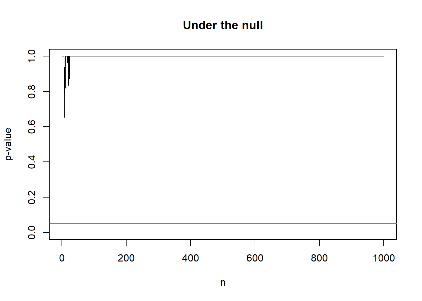
# Under the alternative
alter_out <- sprt_p_value(p_true = 0.6)
plot(seq_along(alter_out$p_val), alter_out$p_val, type = "l",
     xlab = "n", ylab = 'p-value',
     ylim = c(0, 1),
     main = "Under the alternative")
abline(h = alpha, col = 2)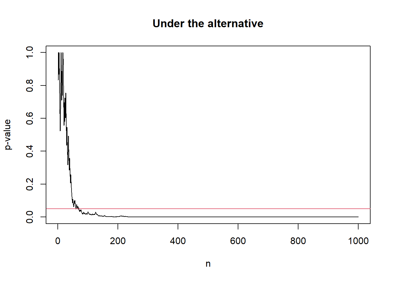
As a remark, the always-valid p-value above is not uniformly distributed. In fact, we can prove that \(p_n \rightarrow 1\) almost surely under the null and \(p_n \rightarrow 0\) almost surely under the alternative as \(n \to \infty\). As it is not uniformly distributed, the standard interpretation of the strength of evidence in terms of p-value is not applicable. In fact, though tracking \(S_n\) and \(p_n\) are equivalent, it is recommended to track \(S_n\) directly as the expectation of \(S_n\) corresponds to the information gain about the difference between null and alternative distributions.
a <- log(1 - beta)
b <- log(1 / alpha)
# Under the null
plot(seq_along(null_out$s), null_out$s, type = "l",
     xlab = "n", ylab = expression('S'['n']),
     main = "Under the null")
abline(h = b, col = 2)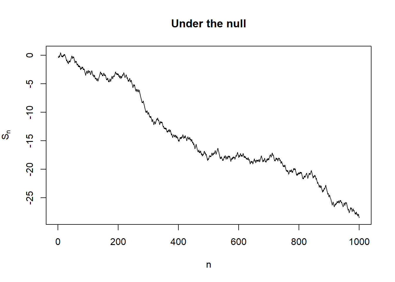
# Under the alternative
plot(seq_along(alter_out$s), alter_out$s, type = "l",
     xlab = "n", ylab = expression('S'['n']),
     main = "Under the alternative")
abline(h = b, col = 2)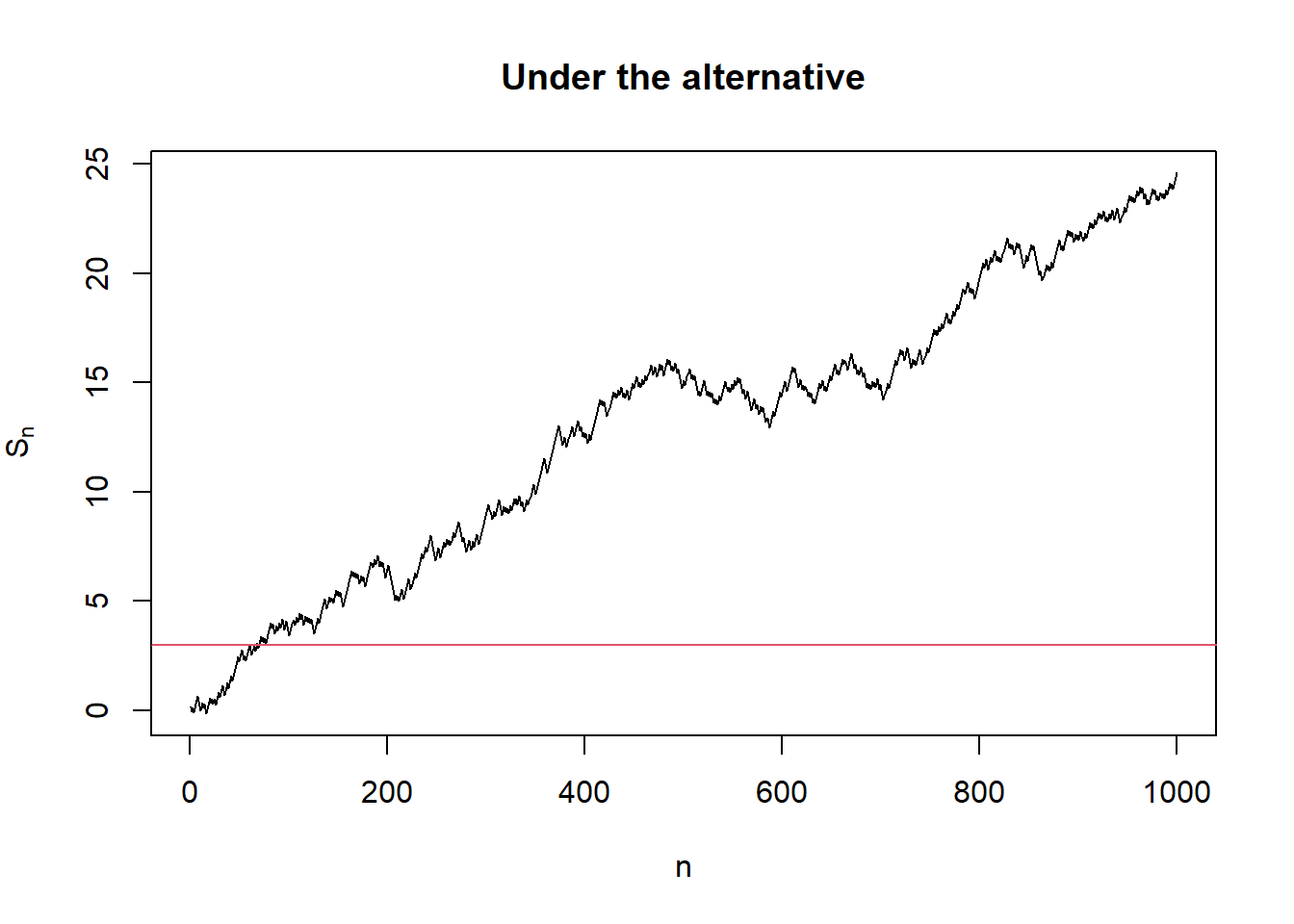
Conclusion
Fixed sample size tests can suffer from type-1 error inflation if the test is not stopped at the pre-specified time. In contrast, sequential hypothesis tests have great flexibility that allows researchers to early stop or continue the experiment without inflating type-1 error.
In fact, in most standard fixed sample tests, we have \(P_{H_0}\left(\exists n: p_n \leq \alpha\right) = 1\).↩︎
Jaehyeok Shin
Data Scientist
Interested in understanding the sequential and adaptive nature of data analysis.