Advantages of Sequential Hypothesis Testing: 1. Sample efficiency

a) Difficulties in sample size calculation in fixed sample size tests

If we know the success probability \(p\) must be equal to a constant \(p_1 > 0.5\) when the coin turns out to be unfair or biased then the Neyman-Pearson lemma shows that for a fixed test level \(\alpha \in (0,1)\), the most powerful test is the likelihood-ratio test (LRT) rejecting the null (\(H_0: p = p_0\)) in a favor of the alternative (\(H_1: p = p_1\)) if \(\bar{X}_n \geq c_\alpha\) where \(\bar{X}_n := \sum_{i=1}^n X_i /n\) and \(c_\alpha\) is a positive constant satisfying \(P_{H_0}(\bar{X}_n \geq c_\alpha) = \alpha\).¹

In fact, LRT is a uniformly most powerful test against all possible alternatives \(p_1\) larger than \(p_0\). Hence, if the sample size and test level are fixed, checking whether the sample mean is larger than the critical value \(c_\alpha\) is all you need to do. This test is also called the exact Binomial test.²

Example R script

set.seed(1)
printf <- function(...) invisible(print(sprintf(...)))
n <- 100L

# Testing fair coin sample (alpha = 0.05)
fair_coin_sample <- rbinom(n, size = 1, prob = 0.5) 
fair_coin_test_result <- binom.test(sum(fair_coin_sample), n, p = 0.5, alternative = "greater")
printf("p-value of a fair coin test is %.3f", fair_coin_test_result$p.value)

## [1] "p-value of a fair coin test is 0.691"

# Testing biased coin sample (alpha = 0.05)
biased_coin_sample <- rbinom(n, size = 1, prob = 0.6)
biased_coin_test_result <- binom.test(sum(biased_coin_sample), n, p = 0.5, alternative = "greater")
printf("p-value of a biased coin test is %.3f", biased_coin_test_result$p.value)

## [1] "p-value of a biased coin test is 0.028"

However, in practice, we rarely know what the alternative success rate could be before an experiment. Instead, we set a minimum effect size of interest \(\Delta > 0\) that we practically consider as a meaningful bias from \(p_0\). Based on the minimum effect size \(\Delta\) and desired minimum power \(\beta \in (0,1)\), we can compute the minimum sample size we need to perform a statistical test that can detect \(p_1 >= p_0 + \Delta\) with probability at least \(\beta\) if the coin is actually biased.

The size of \(\Delta\) depends on the application. For example, If we just play a game at a party with friends, we may still consider a coin with a success probability up to \(0.51\) as a “fairly fair” coin we can use. In this case, the minimum effect size is \(\Delta = 0.1\). On the other hand, if we play a serious gamble with a large bet on the coin toss then even \(0.501\) can be viewed as an unfair coin and the minimum effect size \(\Delta\) is less than \(0.01\).

In any case, since we do not know the “true” alternative \(p_1\), we cannot but set the minimum effect size conservatively. Thus it is possible that the true alternative \(p_1\) turns out to be much larger than the boundary \(p_0 + \Delta\). In this case, the minimum sample size we computed can be very larger than what we could have used to detect the alternative at the same level of detection power.

To detour this issue, it is common practice to conduct a preliminary study with a small sample size to get a rough estimate of \(p_1\) and use it to compute the sample size of the main follow-up study. However, designing a sample efficient preliminary study is itself a non-trivial problem since we cannot reuse samples in the preliminary study for testing the main follow-up experiment.

b) Sequential tests can choose the sample size adaptively.

If there are only two distributions specified in null and alternative hypotheses then similar to the Neyman-Pearson lemma, Wald’s sequential probability ratio test (SPRT) is the test having the smallest average sample size among all statistical tests including both fixed and sequential tests of pre-specified test level \(\alpha\) and minimum power level \(\beta\). It is not contradicting the Neyman-Pearson lemma which only covers all fixed sample size tests. In the sequential test, the sample size is a random stopping time at which we declare whether to reject the null or not.

For our Bernoulli example with \(H_0: p = p_0\) vs \(H_1: p = p_1\), the Wald’s SPRT is given by the following procedure.

• Set \(S_0 := 0\) and for each observation \(X_n\), compute the probability ratio \(\Lambda_n\) by \[ \Lambda_n := \left(\frac{p_1}{p_0}\right)^{X_n}\left(\frac{1-p_1}{1-p_0}\right)^{1-X_n}. \]

• Update \(S_n := S_{n-1} + \log \Lambda_n\)

• Make one of three following decisions:

  • If \(S_n \geq b\) then stop and reject the null (since there is only one alternative, it is equivalent to accept the alternative).

  • If \(S_n \leq a\) then stop and reject the alternative (or accept the null).

  • Otherwise, continue to the next iteration.

Here, thresholds \(a\) and \(b\) are given approximately \(a \sim \log\frac{1-\beta}{1-\alpha}\) and \(b \sim \log\frac{\beta}{\alpha}\) for pre-specified test level \(\alpha\) and minimum power level \(\beta\). Exact thresholds depend on the underlying null and alternative distributions. In the following R example, we use conservative but correct thresholds given by \(a = \log(1-\beta)\) and \(b = \log\frac{1}{\alpha}\).

Example R script for SPRT under the null

set.seed(1)
max_iter <- 1e+3L
p0 <- 0.5 # Null distribution
p1 <- 0.6 # Alternative distribution
alpha <- 0.05 # Test level
beta <- 0.95 # Minimum power level  
a <- log(1 - beta)
b <- log(1 / alpha)
s <- 0
# Set a placeholder only for visualization.
# Actual test does not require it. 

p <- p0 # True distribution is the alternative
s_history <- rep(NA, max_iter) 
for (n in 1:max_iter) {
  # Observe a new sample
  x <- rbinom(1, 1, p)
  # Update S_n
  s <- s + ifelse(x == 1, log(p1/p0), log((1-p1)/(1-p0)))
  s_history[n] <- s
  # Make a decision
  if (s >= b) {
    decision <- "Reject the null"
    break 
  } else if (s <= a) {
    decision <- "Reject the alternative"
    break
  } 
  if (n == max_iter) {
    decision <- "Test reached the max interation"
  }
}
printf("SPRT was ended at n=%i", n)

## [1] "SPRT was ended at n=90"

printf("Decision: %s", decision)

## [1] "Decision: Reject the alternative"

s_history <- s_history[!is.na(s_history)]
plot(seq_along(s_history), s_history, type = "l",
     xlab = "n", ylab = expression('S'['n']),
     ylim = c(a, b))
abline(h = a, col = 2)
abline(h = b, col = 2)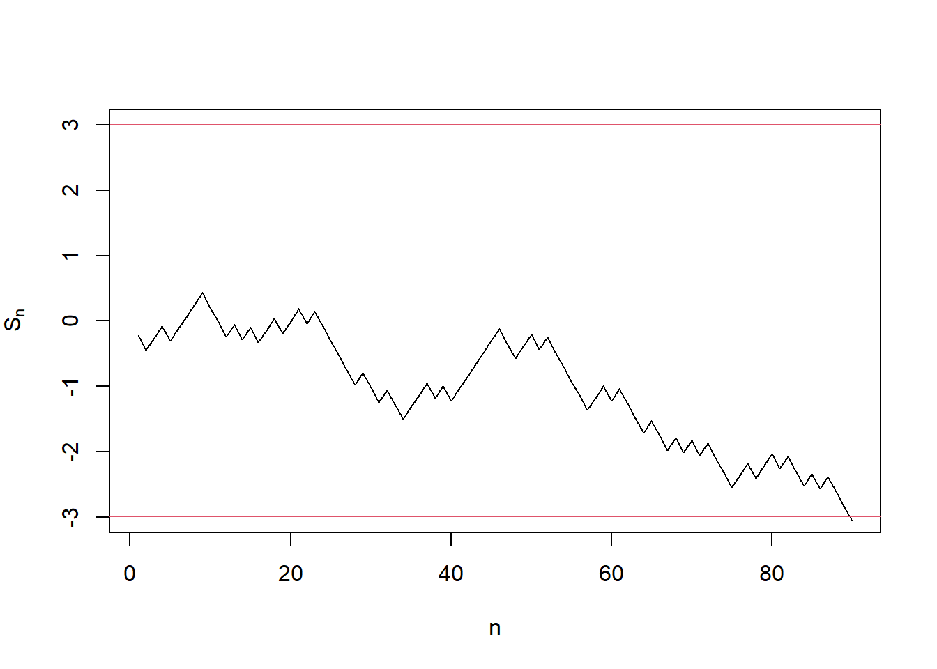

Fig 1. A sample \(S_n\) path of SPRT under the null.

Example R script for SPRT under the alternative

s <- 0
# Set a placeholder only for visualization.
# Actual test does not require it. 
p <- p1 # True distribution is the alternative
s_history <- rep(NA, max_iter) 
for (n in 1:max_iter) {
  # Observe a new sample
  x <- rbinom(1, 1, p)
  # Update S_n
  s <- s + ifelse(x == 1, log(p1/p0), log((1-p1)/(1-p0)))
  s_history[n] <- s
  # Make a decision
  if (s >= b) {
    decision <- "Reject the null"
    break 
  } else if (s <= a) {
    decision <- "Reject the alternative"
    break
  } 
  if (n == max_iter) {
    decision <- "Test reached the max interation"
  }
}
printf("SPRT was ended at n=%i", n)

## [1] "SPRT was ended at n=119"

printf("Decision: %s", decision)

## [1] "Decision: Reject the null"

s_history <- s_history[!is.na(s_history)]
plot(seq_along(s_history), s_history, type = "l",
     xlab = "n", ylab = expression('S'['n']),
     ylim = c(a, b))
abline(h = a, col = 2)
abline(h = b, col = 2)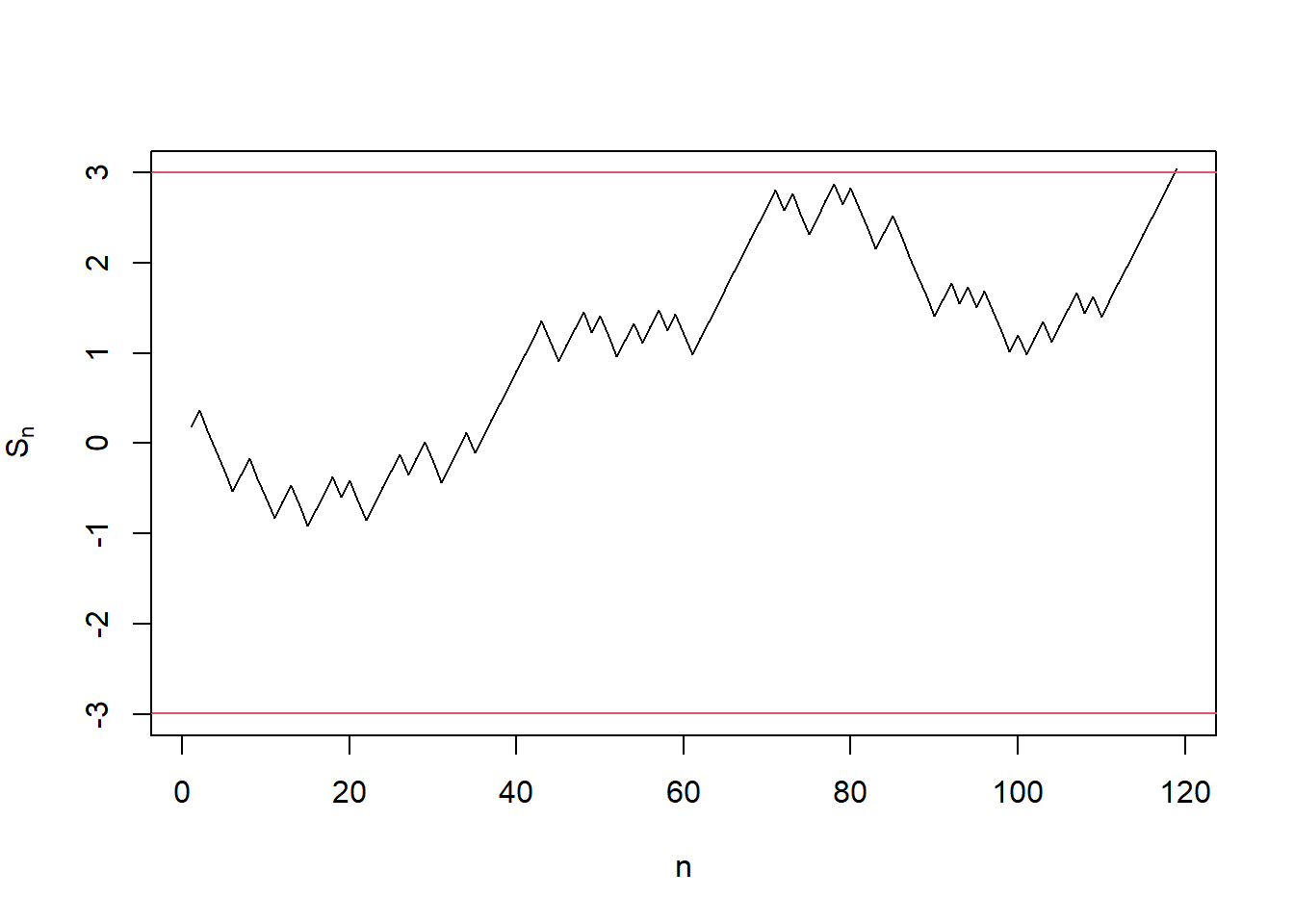

Fig 2. A sample \(S_n\) path of SPRT under the alternative.

From the above example, We can see SPRT ended around \(90\sim120\). However, to achieve the same test level and minimum power, LRT (binomial test in this case), requires at least \(n = 280\) samples.³

Sample size calculation for the Binomial test

n_to_power <- function(n, p0, p1, alpha) {
  n <- ceiling(n)
  thres <- qbinom(alpha, n, p0, lower.tail = FALSE)
  pwr <- pbinom(thres, n, p1, lower.tail = FALSE)
  return(pwr)
}

power_to_n <- function(beta, p0, p1, alpha) {
  f <- function(n) {
    beta - n_to_power(n, p0, p1, alpha)
  }
  root <- stats::uniroot(f, c(1, 1e+4), tol = 1e-6)
  return(ceiling(root$root))
}

alpha <- 0.05
beta <- 0.95
p0 <- 0.5
p1 <- 0.6
minimum_sample <- power_to_n(beta, p0 , p1 , alpha)
printf("%i is the minimum sample size to achieve test level %.2f and power %.2f.", 
       minimum_sample, alpha, beta)

## [1] "280 is the minimum sample size to achieve test level 0.05 and power 0.95."

Unlike the LRT, the efficiency of Wald’s SPRT is guaranteed only for a simple alternative hypothesis space in which there is a single alternative distribution. However, SPRT works reasonably well even for misspecified alternative distributions.⁴

c) Simulations

We end this post by checking the sample efficiency of SPRT over LRT in Bernoulli case simulations. Thoughout the simulation, we use test level \(\alpha = 0.05\), minimum power \(\beta = 0.95\) for hypotheses \(H_0: p = 0.5\) vs \(H_1: p = 0.6\). In this case, the mimum sample size of LRT (one-sided binomial test) is equal to \(n = 280\). Later, we also simulate the misspecified alternatives \(p = 0.55\) and \(p = 0.65\).

Set up

# Set up
alpha <- 0.05
p0 <- 0.5
p1 <- 0.6
beta <- 0.95
n <- power_to_n(beta, p0, p1, alpha) # n = 254
max_iter <- 1e+4L

# One-sided Binomial test 
run_binom_test <- function(n, p_true,
                           p0 = 0.5, p1 = 0.6,
                           alpha = 0.05) {
  thres <- qbinom(alpha, n, p0, lower.tail = FALSE)
  num_head <- rbinom(1, size = n, prob = p_true)
  return(num_head > thres)
}

# SPRT
run_wald_sprt <- function(p_true, p0 = 0.5, p1 = 0.6,
                      alpha = 0.05, beta = 0.95, max_iter = 1e+3L) {
  a <- log(1 - beta)
  b <- log(1 / alpha)
  s <- 0
  for (n in 1:max_iter) {
    # Observe a new sample
    x <- rbinom(1, 1, p_true)
    # Update S_n
    s <- s + ifelse(x == 1, log(p1/p0), log((1-p1)/(1-p0)))
    # Make a decision
    if (s >= b) {
      decision <- "Reject the null"
      is_reject_null <- TRUE
      break 
    } else if (s <= a) {
      decision <- "Reject the alternative"
      is_reject_null <- FALSE
      break
    } 
    if (n == max_iter) {
      decision <- "Test reached the max interation"
      is_reject_null <- FALSE
    }
  } 
  return(list(
    stopped_n = n,
    decision = decision,
    is_reject_null = is_reject_null
  ))
}

set.seed(1)
# Under the null p_true = 0.5
# LRT (binomial)
binom_null_err <- mean(replicate(max_iter, {
  run_binom_test(n, p_true = p0,
                 p0, p1,
                 alpha)
}))
printf("Type 1 error of LRT (n = %i) is %.2f", n, binom_null_err)

## [1] "Type 1 error of LRT (n = 280) is 0.05"

# SPRT 
sprt_null_out <- replicate(max_iter, {
  out <- run_wald_sprt(p_true = p0, p0, p1,
                alpha, beta, max_iter = 1e+3L)
  return(c(stopped_n = out$stopped_n, is_reject_null = out$is_reject_null))
})
sprt_null_err <- mean(sprt_null_out["is_reject_null", ])
sprt_null_sample_size <- mean(sprt_null_out["stopped_n", ])
printf("Type 1 error of SPRT (E[N] = %.1f) is %.2f", sprt_null_sample_size, sprt_null_err)

## [1] "Type 1 error of SPRT (E[N] = 137.7) is 0.04"

set.seed(1)
# Under the alternative p_true = 0.6
# LRT (binomial)
binom_power <- mean(replicate(max_iter, {
  run_binom_test(n, p_true = p1,
                 p0, p1,
                 alpha)
}))
printf("Power of LRT (n = %i) is %.2f", n, binom_power)

## [1] "Power of LRT (n = 280) is 0.96"

# SPRT
sprt_power_out <- replicate(max_iter, {
  out <- run_wald_sprt(p_true = p1, p0, p1,
                       alpha, beta, max_iter = 1e+3L)
  return(c(stopped_n = out$stopped_n, is_reject_null = out$is_reject_null))
})
sprt_power <- mean(sprt_power_out["is_reject_null", ])
sprt_power_sample_size <- mean(sprt_power_out["stopped_n", ])
printf("Power of SPRT (E[N] = %.1f) is %.2f", sprt_power_sample_size, sprt_power)

## [1] "Power of SPRT (E[N] = 139.3) is 0.96"

set.seed(1)
# Under a misspecified alternative 1. small p_true = 0.55.
p_mis1 <- 0.55

# LRT (binomial)
binom_power_mis1 <- mean(replicate(max_iter, {
  run_binom_test(n, p_true = p_mis1,
                 p0, p1,
                 alpha)
}))
printf("Power of LRT (n = %i) is %.2f", n, binom_power_mis1)

## [1] "Power of LRT (n = 280) is 0.52"

# SPRT
sprt_power_mis1_out <- replicate(max_iter, {
  out <- run_wald_sprt(p_true = p_mis1, p0, p1,
                       alpha, beta, max_iter = 1e+3L)
  return(c(stopped_n = out$stopped_n, is_reject_null = out$is_reject_null))
})
sprt_power_mis1 <- mean(sprt_power_mis1_out["is_reject_null", ])
sprt_power_mis_1_sample_size <- mean(sprt_power_mis1_out["stopped_n", ])
printf("Power of SPRT (E[N] = %.1f) is %.2f", sprt_power_mis_1_sample_size, sprt_power_mis1)

## [1] "Power of SPRT (E[N] = 234.5) is 0.50"

set.seed(1)
# Under a misspecified alternative 2. large p_true = 0.65.
p_mis2 <- 0.65

# LRT (binomial)
binom_power_mis2 <- mean(replicate(max_iter, {
  run_binom_test(n, p_true = p_mis2,
                 p0, p1,
                 alpha)
}))
printf("Power of LRT (n = %i) is %.2f", n, binom_power_mis2)

## [1] "Power of LRT (n = 280) is 1.00"

sprt_power_mis2_out <- replicate(max_iter, {
  out <- run_wald_sprt(p_true = p_mis2, p0, p1,
                       alpha, beta, max_iter = 1e+3L)
  return(c(stopped_n = out$stopped_n, is_reject_null = out$is_reject_null))
})
sprt_power_mis2 <- mean(sprt_power_mis2_out["is_reject_null", ])
sprt_power_mis_2_sample_size <- mean(sprt_power_mis2_out["stopped_n", ])
printf("Power of SPRT (E[N] = %.1f) is %.2f", sprt_power_mis_2_sample_size, sprt_power_mis2)

## [1] "Power of SPRT (E[N] = 76.1) is 1.00"

Conclusion

Sequential hypothesis testing procedures can achieve a better sample efficiency even compared to the best-fixed sample size test. In the following post, we will explain the flexibility and safety of sequential testing procedures.